What is a Full Factorial DOE?
In a full factorial experiment, all of the possible combinations of factors and levels are created and tested. For example, for two-level design (i.e.each factor has two levels) with k factors, there are 2k possible scenarios or treatments.
- Two factors, each with two levels, we have 22 = 4 treatments
- Three factors, each with two levels, we have 23 = 8 treatments
- k factors, each with two levels, we have 2k treatments
2k Full Factorial DOE
Full factorial DOE is used to discover the cause-and-effect relationship between the response and both individual factors and the interaction of factors. Generate an equation to describe the relationship between Y and the important Xs:
![]()
Where:
- Y is the response and X1, X2 . . . Xk are the factors
- α0 is the intercept and α1, α2 . . . αp are the coefficients of the factors and interactions
- ε is the error of the model
Two-Level Two-Factor Full Factorial
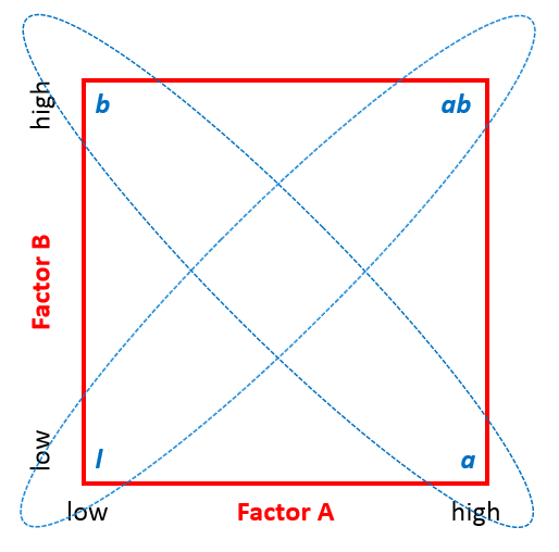
Below is a design pattern of a two-level two-factor full factorial experiment.
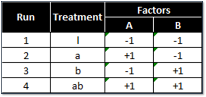
2 (level) raised to 2 (factors) = 4 treatment combinations.
Two-Level Three-Factor Full Factorial
Below is a design pattern of a two-level three-factor full factorial experiment.
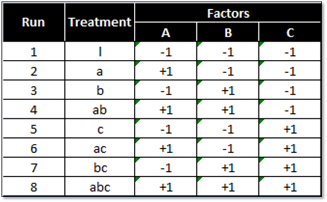
2 (levels) raised to 3 (factors) = 8 treatment combinations.
Two-Level Four-Factor Full Factorial
Below is a design pattern of a two-level four-factor full factorial experiment
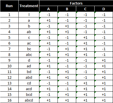
2 (levels) raised to 4 (factors) = 16 treatment combinations
Two-Level Five-Factor Full Factorial
Below is a design pattern of a two-level five-factor full factorial experiment
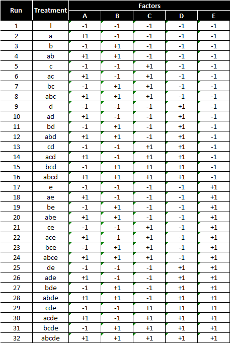
2 (levels) raised to 5 (factors) = 32 treatment combinations
Order to Run Experiments
The four design patterns shown earlier are listed in the standard order. Standard order is used to design the combinations/treatments before experiments start. When actually running the experiments, randomizing the standard order is recommended to minimize the noise.
Replication in Experiments
Each treatment can be tested multiple times in an experiment in order to increase the degrees of freedom and improve the capability of analysis. We call this method replication.
Replicates are the number of repetitions of running an individual treatment, which increase the power of the experimental responses. The order to run the treatments in an experiment should be randomized to minimize the noise.
Advantages of replication include: helps to better identify the true sources of variation, helps estimate the true impacts of the factors on the response, and overall improves the reliability and validity of the experimental results.
22 Full Factorial DOE
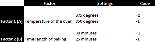
Case study: We are running a 22 full factorial DOE to discover the cause-and-effect relationship between the cake tastiness and two factors: temperature of the oven and time length of baking. Each factor has two levels and there are four treatments in total.
We decide to run each treatment twice so that we have enough degrees of freedom to measure the impact of two factors and the interaction between two factors. Therefore, there are eight observations in response eventually.
The objective is to understand the main effects and the interactions of these factors on the response variable. After running the four treatments twice in a random order, we obtain the following results
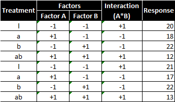
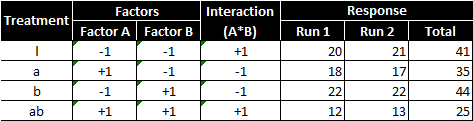
There are two factors and two levels, so there would be 2^2 = 4 treatment combinations. With replicates, each treatment combination is repeated once; therefore, there are in total 8 runs in this experiment. The experiment results are consolidated into the following table
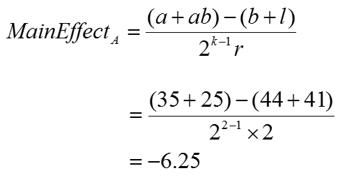
The main effect of factor A is computed by averaging the difference between combinations where A was at its high settings and where A was at its low settings.
Main effect of factor A (temperature of the oven):
Where:
- k is the number of factors
- r is the number of times individual treatments are being run
Using the formula provided, the main effect of increasing the temperature of the oven is to decrease tastiness of the cake by −6.25.
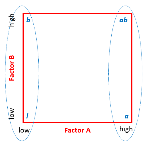
The main effect of factor B, similar to A, is computed by averaging the difference between combinations where B was at its high settings and where B was at its low settings.
Main effect of factor B (time length of baking):
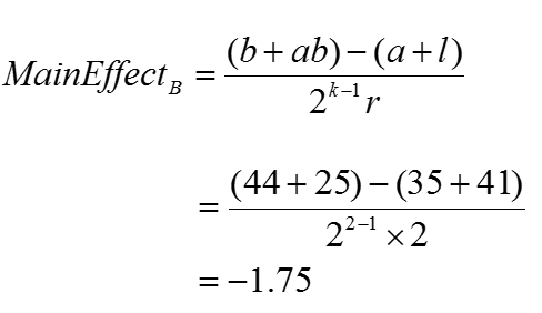
Where:
- k is the number of factors
- r is the number of times individual treatments are being run
Using the formula provided, the main effect of increasing the baking time is to decrease the tastiness of the cake by −1.75
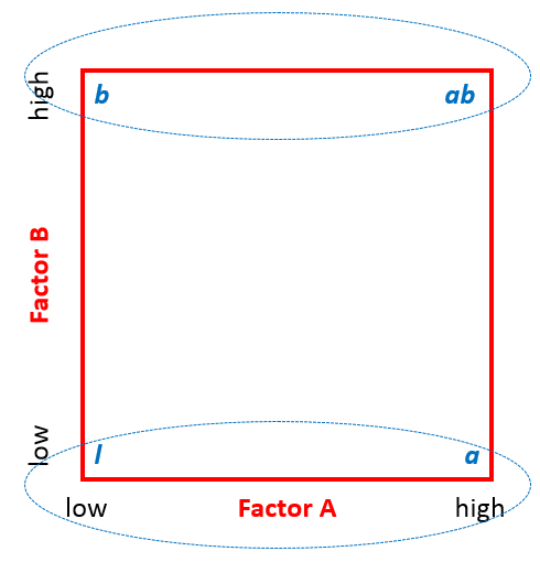
The interaction effect is computed by averaging the difference between combinations where A and B were at opposite settings (low and high).
Interaction (i.e. A*B) effect:
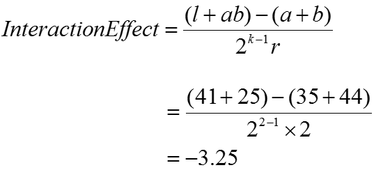
Where:
- k is the number of factors
- r is the number of times individual treatments are being run
Using the formula provided, the interaction effect of the temperature and time variables on tastiness was −3.25.
Sum of squares of factors and interaction
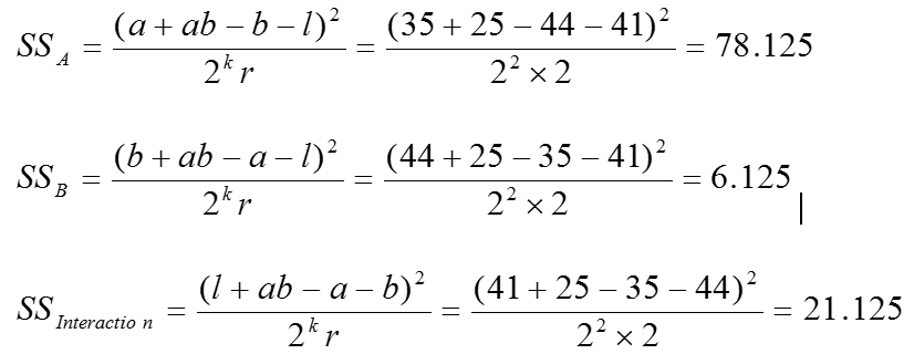
Where:
- k is the number of factors
- r is the number of times individual treatments are being run
The sum of squares tells us the relative strength of each main effect and interaction. A has the strongest effect as indicated by the high SS value. The degrees of freedom are necessary to determine the mean squares value.
Degrees of freedom of factors and interaction:
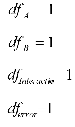
Four degrees of freedom are necessary because there are three effects we are looking to understand: factor A, factor B, and the interaction between them.
![]()
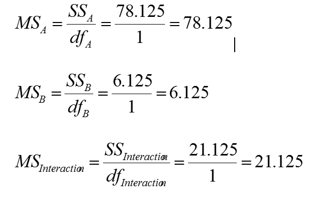
Mean squares of factors and interaction:
Use Minitab to Run a 2k Full Factorial DOE
Step 1: Initiate the experiment design
- Click Stat → DOE → Factorial → Create Factorial Design.
- A new window named “Create Factorial Design” pops up.
- Select the button of “General full factorial design.”
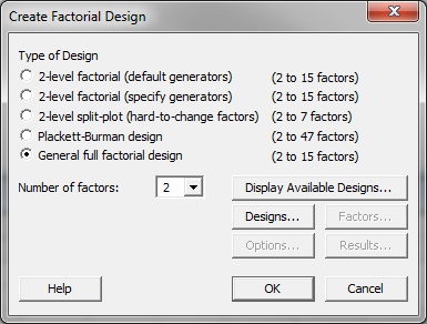
- Select “2” as the “Number of factors.”
- Click the “Design” button and a new window named “Create Factorial Design – Designs” pops up.
- Enter the factor name “Temperature” for factor A.
- Enter the factor name “Time Length” for factor B.
- Enter the number of levels “2” for both factor A and B.
- Enter “2” as the “Number of replicates.
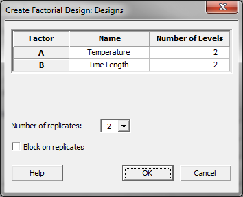
- Click “OK” button in the window “Create Factorial Design – Designs.”
Step 2: Enter the factors and make the design
- Click on the “Factors” button in the window “Create Factorial Design”
- A new window named “Create Factorial Design – Factors” pops up.
- Select “Text” as the “Type” of both factor A and B.
- Enter “Low” and “High” as the two levels for both factor A and B.
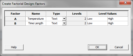
- Click “OK” in the window “Create Factorial Design – Factors.”
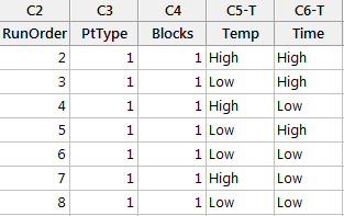
- Click “OK” in the window “Create Factorial Design.”
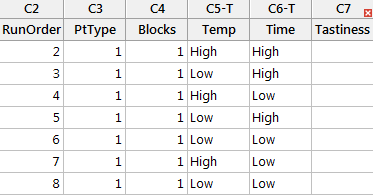
- The design table is created in the data table.
Step 3: Run your experiment and record the response for each run in a new column named Tastiness within the table created by Minitab. Because we are simulating a DOE we have provided the data for you in the Sample Data.xlsx file. Use this data to populate your table with your experiment results
Step 4: Analyze the experiment results
- Click Stat → DOE → Factorial → Analyze Factorial Design.
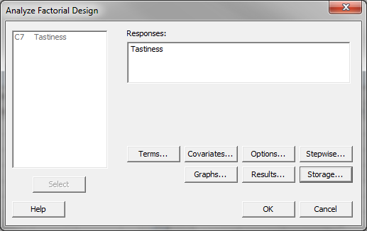
- A new window named “Analyze Factorial Design” appears.
- Select “Tastiness” in the list box of “Responses.”
- Click on the “Storage” button and a new window named “Analyze Factorial Design – Storage” pops up.
- Check the boxes “Fits” and “Residuals” in the window “Analyze Factorial Design – Storage.”
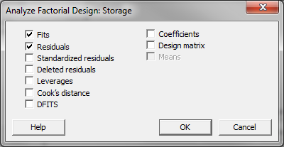
- Click “OK” in the window “Analyze Factorial Design – Storage.”
- Click “OK” in the window “Analyze Factorial Design.”
- The DOE analysis results appear in the session window.
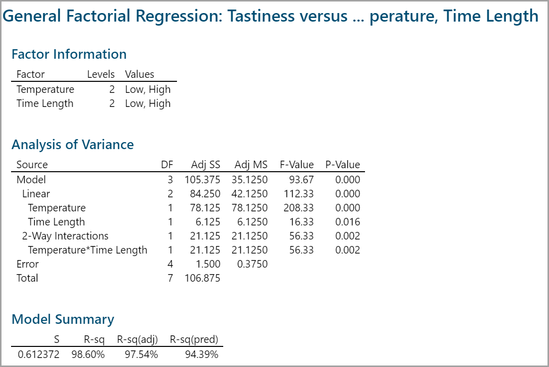
These are the results.
Since the p-values of all the independent variables in the model are smaller than the alpha level (0.05), both factors and their interactions have statistically significant impact on the response.
High R2 value shows around 98% of the variation in the response can be explained by the model (very good results).
The fitted response and the residuals of the DOE model are stored in the last two columns of the data table.
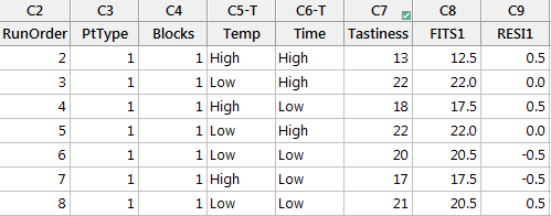 Model summary: These are the software outputs for expected/predicted results, as well as the residuals for each combination.
Comments are closed.